Long description: heatexample
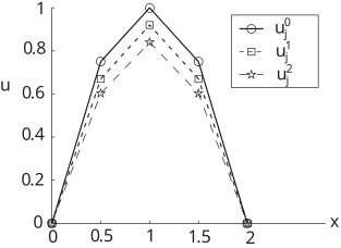
Alt text: A line graph illustrates the temperature distribution, represented by \(u\), across a length \(x\), showing three different solutions, \(u_j^0\), \(u_j^1\), and \(u_j^2\), at time \(t=1\) and \(t=2\).
This description was generated by AI and has not been verified by a human. If you spot an error, please use the feedback link below.
- The graph displays three curves, labeled \(u_j^0\) (circles), \(u_j^1\) (squares), and \(u_j^2\) (stars), plotting a value \(u\) on the vertical axis against a position \(x\) on the horizontal axis, ranging from \(0\) to \(2\).
- All three solutions start at \(u=0\) when \(x=0\) and end at \(u=0\) when \(x=2\).
- The curve \(u_j^0\) reaches its maximum value at \(x=1\), where \(u \text{ equals } 1\).
- The curve \(u_j^1\) also reaches its maximum value at \(x=1\), where \(u\) is slightly below \(1\).
- The curve \(u_j^2\) also peaks at \(x=1\), with a value slightly below \(u_j^1\).
- At \(x=0.5\), the values are approximately \(u_j^0 = 0.7\), \(u_j^1 = 0.6\), and \(u_j^2 = 0.55\).
- At \(x=1.5\), the values are approximately \(u_j^0 = 0.7\), \(u_j^1 = 0.6\), and \(u_j^2 = 0.55\), reflecting symmetry around \(x=1\).