2 Finding the gradient at a specific point

In this subsection we shall consider a simple function to illustrate the calculation of a gradient. Look at the graph of the function $y\left(x\right)=x^2$ shown in Figure 4. Notice that the gradient of the graph changes as we move from point to point. In some places the gradient is positive; at others it is negative. The gradient is greater at some points than at others. In fact the gradient changes from point to point as we move along the curve.

Figure 4

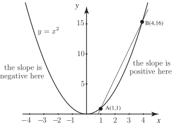
Inspect the graph carefully and make the following observations:

1. $A$ is the point with coordinates $\left(1,1\right)$ .
2. $B$ is the point with coordinates $\left(4,16\right)$ .
3. We can calculate the gradient of the line $AB$ from the formula
   $$\text{ gradient }=\frac{\text{ difference between }y\text{ coordinates}}{\text{ difference between }x\text{ coordinates}}$$
   Therefore the gradient of chord $AB$ is equal to $\frac{16-1}{4-1}=\frac{15}{3}=5$ . The gradient of $AB$ is not the same as the gradient of the graph at $A$ but we can regard it as an approximation, or estimate of the gradient at $A$ . Is it an over-estimate or under-estimate ?

Task!

Add the point $C$ to the graph in Figure 4 where $C$ has coordinates $\left(3,9\right)$ . Draw the line $AC$ and calculate its gradient.

Answer

We now carry the last task further by introducing point $D$ at $\left(2,4\right)$ and point $E$ at $\left(1.5,2.25\right)$ as shown in Figure 5. The gradient of $AD$ is found to be 3 and the gradient of $AE$ is 2.5.

Figure 5

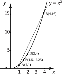
Observe that each time we carry out this procedure, and move the second point closer to $A$ , the gradient of the line drawn is getting closer and closer to the gradient of the tangent at $A$ . If we continue, the value we eventually obtain is the gradient of the tangent at $A$ whose value is 2 as we will see shortly. This procedure illustrates how we define the gradient of the curve at $A$ .