1 The second shift theorem

The second shift theorem is similar to the first except that, in this case, it is the time-variable that is shifted not the s -variable. Consider a causal function f ( t ) u ( t ) which is shifted to the right by amount a , that is, the function f ( t − a ) u ( t − a ) where a > 0 . Figure 13 illustrates the two causal functions.

Figure 13
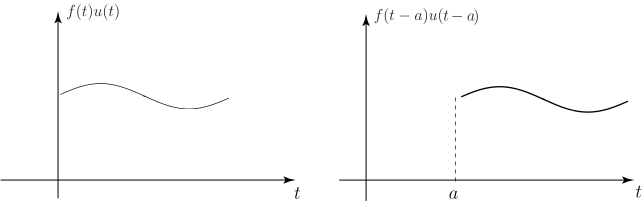
The image displays two graphs illustrating the time-shifting property of the Fourier transform: the left graph shows \(f(t)u(t)\) and the right graph shows \(f(t-a)u(t-a)\).

Long description

The Laplace transform of the shifted function is easily obtained:

L { f ( t − a ) u ( t − a ) } = ∫ 0 ∞ e − s t f ( t − a ) u ( t − a ) d t = ∫ a ∞ e − s t f ( t − a ) d t

(Note the change in the lower limit from 0 to a resulting from the step function switching on at t = a ). We can re-organise this integral by making the substitution x = t − a . Then d t = d x and when t = a , x = 0 and when t = ∞ then x = ∞ .

Therefore

∫ a ∞ e − s t f ( t − a ) d t = ∫ 0 ∞ e − s ( x + a ) f ( x ) d x = e − s a ∫ 0 ∞ e − s x f ( x ) d x

The final integral is simply the Laplace transform of f ( x ) , which we know is F ( s ) and so, finally, we have the statement of the second shift theorem:

Key Point 8

Second Shift Theorem

If L { f ( t ) } = F ( s ) then L { f ( t − a ) u ( t − a ) } = e − s a F ( s )

Obviously, this theorem has its uses in finding the Laplace transform of time-shifted causal functions but it is also of considerable use in finding inverse Laplace transforms since, using the inverse formulation of the theorem of Key Point 8 we get:

Key Point 9

Inverse Second Shift Theorem

If L − 1 { F ( s ) } = f ( t ) then L − 1 { e − s a F ( s ) } = f ( t − a ) u ( t − a )

Task!

Find the inverse Laplace transform of e − 3 s s 2 .

You should obtain ( t − 3 ) u ( t − 3 ) for the following reasons. We know that the inverse Laplace transform of 1 ∕ s 2 is t . u ( t ) (Table 1, Rule 3) and so, using the second shift theorem (with a = 3 ), we have

L − 1 { e − 3 s 1 s 2 } = ( t − 3 ) u ( t − 3 )

This function is graphed in the following figure:
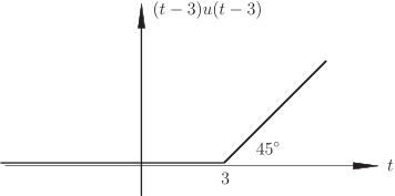
A graph showing a line segment starting at the point (3, 0) and extending upwards with a slope of 45 degrees.

Long description
Task!

Find the inverse Laplace transform of s s 2 − 2 s + 2

You should obtain e t ( cos t + sin t ) .

To obtain this, complete the square in the denominator: s 2 − 2 s + 2 = ( s − 1 ) 2 + 1 and so

s s 2 − 2 s + 2 = s ( s − 1 ) 2 + 1 = ( s − 1 ) + 1 ( s − 1 ) 2 + 1 = s − 1 ( s − 1 ) 2 + 1 + 1 ( s − 1 ) 2 + 1

Now, using the first shift theorem

L − 1 { s − 1 ( s − 1 ) 2 + 1 } = e t cos t . u ( t )  since L − 1 { s s 2 + 1 } = cos t . u ( t )  (Table 1, Rule 6)

and

L − 1 { 1 ( s − 1 ) 2 + 1 } = e t sin t . u ( t )  since L − 1 { 1 s 2 + 1 } = sin t . u ( t )  (Table 1. Rule 5)

Thus

L − 1 { s s 2 − 2 s + 2 } = e t ( cos t + sin t ) u ( t )