3 The delta function (or impulse function)

There is often a need for considering the effect on a system (modelled by a differential equation) by a forcing function which acts for a very short time interval. For example, how does the current in a circuit behave if the voltage is switched on and then very shortly afterwards switched off? How does a cantilevered beam vibrate if it is hit with a hammer (providing a force which acts over a very short time interval)? Both of these engineering ‘systems’ can be modelled by a differential equation. There are many ways the ‘kick’ or ‘impulse’ to the system can be modelled. The function we have in mind could have the graphical representation (when $a$ is small) shown in Figure 14.

Figure 14

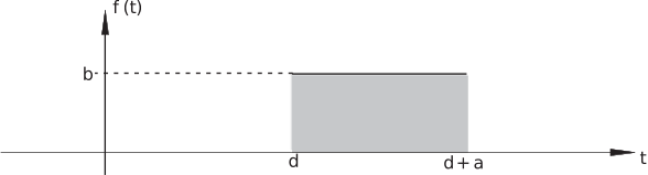
This can be represented formally using step functions; it switches on at $t=d$ and switches off at $t=d+a$ and has amplitude $b$ :

$f\left(t\right)=b\left[u\left(t-d\right)-u\left(t-\left\{d+a\right\}\right)\right]$

The effect on the system is related to the area under the curve rather than just the amplitude $b$ . Our aim is to reduce the time interval over which the forcing function acts (i.e. reduce $a$ ) whilst at the same time keeping the total effect (i.e. the area under the curve) a constant. To do this we shall take $b=1∕a$ so that the area is always equal to 1. Reducing the value of $a$ then gives the sequence of inputs shown in Figure 15.

Figure 15

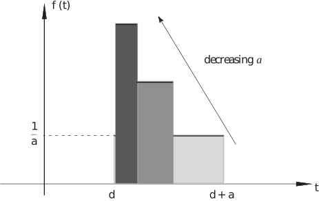
As the value of $a$ decreases the height of the rectangle increases (to ensure the value of the area under the curve is fixed at value 1) until, in the limit as $a\to 0$ , the ‘function’ becomes a ‘spike’ at $t=d$ . The resulting function is called a delta function (or impulse function ) and denoted by $\delta \left(t-d\right)$ . This notation is used because, in a very obvious sense, the delta function described here is ‘located’ at $t=d$ . Thus the delta function $\delta \left(t-1\right)$ is ‘located’ at $t=1$ whilst the delta function $\delta \left(t\right)$ is ‘located’ at $t=0$ .

If we were defining an ordinary function we would write

$\delta \left(t-d\right)=\underset{a\to 0}{lim}\frac{1}{a}\left[u\left(t-d\right)-u\left(t-\left\{d+a\right\}\right)\right]$

However, this limit does not exist. The important property of the delta function relates to its integral:

which is what we expect since the area under each of the limiting curves is equal to $1$ .

A more technical discussion obtains the more general result:

This is called the sifting property of the delta function as it sifts out the value $f\left(d\right)$ from the function $f\left(t\right)$ . Although the integral here ranges from $t=-\infty$ to $t=+\infty$ in fact the same result is obtained for any range if the range of the integral includes the point $t=d$ . That is, if $\alpha \le d\le \beta$ then

${\int \; <!--nolimits\; -->}_{\alpha }^{\beta }f\left(t\right)\delta \left(t-d\right)dt=f\left(d\right)$

Thus, as long as the delta function is ‘located’ within the range of the integral the sifting property holds. For example,

${\int \; <!--nolimits\; -->}_1^{2}sint\delta \left(t-1.1\right)dt=sin1.1=0.8112{\int \; <!--nolimits\; -->}_0^{\infty }{\text{e}}^{-t}\delta \left(t-1\right)dt={\text{e}}^{-1}=0.3679$

Task!

Write expressions for delta functions located at $t=-1.7$ and at $t=2.3$

Answer

Task!

Evaluate the integral ${\int \; <!--nolimits\; -->}_{-1}^3\left(sint\delta \left(t+2\right)-cost\delta \left(t\right)\right)dt$

Answer

3.1 The Laplace transform of the delta function

Here we consider $\mathcal{L}\left\{\delta \left(t-d\right)\right\}$ . From the definition of the Laplace transform:

$\mathcal{L}\left\{\delta \left(t-d\right)\right\}={\int \; <!--nolimits\; -->}_0^{\infty }{\text{e}}^{-st}\delta \left(t-d\right)dt={\text{e}}^{-sd}$

by the sifting property of the delta function. Thus

Exercise

Find the Laplace transforms of   $3\delta \left(t-3\right).$

Answer

$3e^{-3s}$