1 Sampling theory

If a continuous-time signal $f\left(t\right)$ is sampled at terms $t=0,T,2T,\dots nT,\dots$ then a sequence of values

$\left\{f\left(0\right),f\left(T\right),f\left(2T\right),\dots f\left(nT\right),\dots \right\}$

is obtained. The quantity $T$ is called the sample interval or sample period .

Figure 18

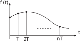
In the previous Sections of this Workbook we have used the simpler notation $\left\{f_n\right\}$ to denote a sequence. If the sequence has actually arisen by sampling then $f_n$ is just a convenient notation for the sample value $f\left(nT\right)$ .

Most of our previous results for z-transforms of sequences hold with only minor changes for sampled signals.

So consider a continuous signal $f\left(t\right)$ ; its z-transform is the z-transform of the sequence of sample values i.e.

$\mathbb{Z}\left\{f\left(t\right)\right\}=\mathbb{Z}\left\{f\left(nT\right)\right\}={\sum }_{n=0}^{\infty }f\left(nT\right)z^{-n}$

We shall briefly obtain z-transforms of common sampled signals utilizing results obtained earlier. You may assume that all signals are sampled at $0,T,2T,\dots nT,\dots$

Unit step function

$u\left(t\right)=\left\{\begin{array}{cc}\hfill 1\hfill & \hfill t\ge 0\hfill \\ \hfill 0\hfill & \hfill t<0\hfill \end{array}\right.$

Since the sampled values here are a sequence of 1’s,

where $\left\{u_n\right\}=\left\{1,1,1,\dots \right\}$ is the unit step sequence.

$\uparrow$

Ramp function

$r\left(t\right)=\left\{\begin{array}{ccc}t\hfill & \hfill \hfill & t\ge 0\hfill \\ 0\hfill & \hfill \hfill & t<0\hfill \end{array}\right.$

The sample values here are

$\left\{r\left(nT\right)\right\}=\left\{0,T,2T,\dots \right\}$

The ramp sequence   $\left\{r_n\right\}=\left\{0,1,2,\dots \right\}$  has z-transform $\frac{z}{{\left(z-1\right)}^2}$ .

Hence $\mathbb{Z}\left\{r\left(nT\right)\right\}=\frac{Tz}{{\left(z-1\right)}^2}$  since $\left\{r\left(nT\right)\right\}=T\left\{r_n\right\}$ .

Task!

Obtain the z-transform of the exponential signal

$f\left(t\right)=\left\{\begin{array}{ccc}{e}^{-\alpha t}\hfill & \hfill \hfill & t\ge 0\hfill \\ 0\hfill & \hfill \hfill & t<0.\hfill \end{array}\right.$

[Hint: use the z-transform of the geometric sequence $\left\{a^n\right\}$ .]

Answer

Earlier in this Workbook we obtained the z-transform of the sequence $\left\{cos\omega n\right\}$ i.e.

$\mathbb{Z}\left\{cos\omega n\right\}=\frac{z^2-zcos\omega }{z^2-2zcos\omega +1}$

Hence, since sampling the continuous sinusoid

$f\left(t\right)=cos\omega t$

yields the sequence $\left\{cosn\omega T\right\}$ we have, simply replacing $\omega$ by $\omega T$ in the z-transform:

Task!

Obtain the z-transform of the sampled version of the sine wave $f\left(t\right)=sin\omega t$ .

Answer

These are similar to those discussed earlier in this Workbook but for sampled signals the shifts are by integer multiples of the sample period $T$ . For example a simple right shift, or delay, of a sampled signal by one sample period is shown in the following figure:

Figure 19

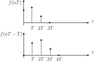
The right shift properties of z-transforms can be written down immediately. (Look back at the shift properties in Section 21.2 subsection 5, if necessary:)

If $y\left(t\right)$ has z-transform $Y\left(z\right)$ which, as we have seen, really means that its sample values $\left\{y\left(nT\right)\right\}$ give $Y\left(z\right)$ , then for $y\left(t\right)$ shifted to the right by one sample interval the $z$ -transform becomes

$\mathbb{Z}\left\{y\left(t-T\right)\right\}=y\left(-T\right)+z^{-1}Y\left(z\right)$

The proof is very similar to that used for sequences earlier which gave the result:

$\mathbb{Z}\left\{y_{n-1}\right\}=y_{-1}+z^{-1}Y\left(z\right)$

Task!

Using the result

$\mathbb{Z}\left\{y_{n-2}\right\}=y_{-2}+y_{-1}{z}^{-1}+z^{-2}Y\left(z\right)$

write down the result for $\mathbb{Z}\left\{y\left(t-2T\right)\right\}$

Answer

These results can of course be generalised to obtain $\mathbb{Z}\left\{y\left(t-mT\right)\right\}$ where $m$ is any positive integer.

In particular, for causal or one-sided signals $y\left(t\right)$ (i.e. signals which are zero for $t<0$ ):

$\mathbb{Z}\left\{y\left(t-mT\right)\right\}=z^{-m}Y\left(z\right)$

Note carefully here that the power of $z$ is still $z^{-m}$ not $z^{-mT}$ . Examples:

For the unit step function we saw that:

$\mathbb{Z}\left\{u\left(t\right)\right\}=\frac{z}{z-1}=\frac{1}{1-z^{-1}}$

Hence from the shift properties above we have immediately, since $u\left(t\right)$ is certainly causal,

and so on.

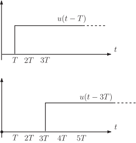
Figure 20