2 Partial differential equations
In all the above examples we had a function of a single variable being the solution of an ordinary differential equation.
In engineering and science ODEs arise as models for systems where there is one independent variable (often ) and one dependent variable (often ). Obvious examples are lumped electrical circuits where the current is a function only of time (and not of position in the circuit) and lumped mechanical systems (such as the simple harmonic oscillator referred to above) where the displacement of a moving particle depends only on .
However, in problems where one variable, say , depends on more than one independent variable, say both and , then any derivatives of will be partial derivatives such as or and any differential equation arising will be known as a partial differential equation. In particular, one-dimensional (1-D) time-dependent problems where depends on a position coordinate and the time and two-dimensional (2-D) time-independent problems where is a function of the two position coordinates and both give rise to PDEs involving two independent variables. This is the case we shall concentrate on. A two-dimensional time-dependent problem would involve 3 independent variables as would a three-dimensional time-independent problem where would be the independent variables.
Example 1
Show that satisfies the PDE .
This PDE is known as Laplace’s equation in two dimensions and it arises in many applications e.g. electrostatics, fluid flow, heat conduction.
Solution
Differentiating again gives
Hence
so the given function is indeed a solution of the PDE.
Task!
Show that is a solution of the PDE
First find and :
Now find and complete the Task:
and we see that as required.
The PDE in the above Task has the general form
where is a positive constant. This equation is referred to as the one-dimensional heat conduction equation (or sometimes as the diffusion equation ). In a heat conduction context the dependent variable represents the temperature .
The third important PDE involving two independent variables is known as the one-dimensional wave equation . This has the general form
(Note that both partial derivatives in the wave equation are second-order in contrast to the heat conduction equation where the time derivative is first order.)
Example 2
- Verify that (where and are constants) satisfies the one-dimensional wave equation.
- Verify the boundary conditions i.e. .
- Verify the initial conditions i.e. and .
- Give a physical interpretation of this problem.
-
By straightforward partial differentiation of the given function
:
We see that which completes the verification.
-
Putting
, and leaving
arbitrary, in the given solution for
gives
Similarly putting arbitrary:
-
Evaluating
firstly for general
and
Now putting leaving arbitrary
Also, putting in the expression for gives
-
Mathematically we have now proved that the given function
satisfies the
-D wave equation specified in 1., the two
boundary conditions
specified in 2. and the two
initial conditions
specified in 3.
One possible physical interpretation of this problem is that represents the displacement of a string stretched between two points at and . Clearly the position of any point on the vibrating string will depend upon its distance from one end and on the time .
The boundary conditions 2. represent the fact that the string is fixed at these end-points.
The initial condition represents the displacement of the string at .
The initial condition tells us that the string is at rest at .
Figure 1
Long description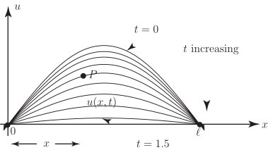
Note that it can be proved formally that if is the tension in the string and if is the mass per unit length of the string then does, under certain conditions, satisfy the -D wave equation with .
Key Point 4
The three PDEs of greatest general interest involving two independent variables are:
-
The two-dimensional Laplace equation
-
The one-dimensional heat conduction equation:
-
The one-dimensional wave equation: