1 Cauchy’s theorem
1.1 Simply-connected regions
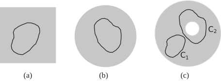
A region is said to be simply-connected if any closed curve in that region can be shrunk to a point without any part of it leaving a region. The interior of a square or a circle are examples of simply connected regions. In Figure 11 (a) and (b) the shaded grey area is the region and a typical closed curve is shown inside the region. In Figure 11 (c) the region contains a hole (the white area inside). The shaded region between the two circles is not simply-connected; curve can shrink to a point but curve cannot shrink to a point without leaving the region, due to the hole inside it.
Figure 11
Key Point 2
Cauchy’s Theorem
The theorem states that if is analytic everywhere within a simply-connected region then:
for every simple closed path lying in the region.
This is perhaps the most important theorem in the area of complex analysis.
As a straightforward example note that , where is the unit circle, since is analytic everywhere (see Section 261). Indeed for any simple contour: it need not be circular.
Consider the contour shown in Figure 12 and assume is analytic everywhere on and inside the contour .
Figure 12
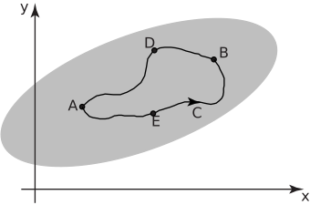
Then by analogy with real line integrals
by Cauchy’s theorem.
Therefore
(since reversing the direction of integration reverses the sign of the integral).
This implies that we may choose any path between and and the integral will have the same value providing is analytic in the region concerned.
Integrals of analytic functions only depend on the positions of the points and , not on the path connecting them. This explains the ‘coincidences’ referred to previously in Section 26.4.
Task!
Using ‘simple’ integration evaluate , and explain why this is valid.
.
This way of determining the integral is legitimate because is analytic (everywhere).
We now investigate what occurs when the closed path of integration does not necessarily lie within a simply-connected region. Consider the situation described in Figure 13.
Figure 13
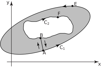
Let be analytic in the region bounded by the closed curves and . The region is cut by the line segment joining and .
Consider now the closed curve travelling in the direction indicated by the arrows. No line can cross the cut and be regarded as remaining in the region. Because of the cut the shaded region is simply connected . Cauchy’s theorem therefore applies (see Key Point 2).
Therefore
since is analytic within and on the curve .
Note that
being a simple change of direction.
Also, we can divide the closed curve into smaller sections:
i.e.
(since we assume that closed paths are travelled anticlockwise).
Therefore .
This allows us to evaluate by replacing by any curve such that the region between them contains no singularities (see Section 261) of . Often we choose a circle for .
Example 12
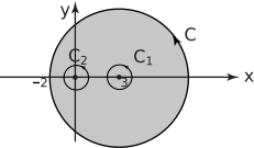
Determine where is the curve shown in Figure 14.
Figure 14
Solution
We observe that is analytic everywhere except at and .
Let be the circle of unit radius centred at and be the unit circle centered at the origin. By analogy with the previous example we state that
(To show this you would need two cuts: from to and from to .)
The remaining parts of this problem are presented as two Tasks.
Task!
Expand into partial functions.
Let . Then
If
Thus:
Task!
Find the values of , using Key Point 1 (page 35):
-
Find the value of
:
Using Key Point 1 we find that .
-
Find the value of
:
The function is analytic inside and on so that .
-
Find the value of
:
The function is analytic inside and on so .
-
Find the value of
:
again using Key Point 1.
-
Finally, calculate
:
Exercises
- Evaluate
- Determine where is the contour
- since is analytic everywhere.
-
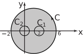
is analytic everywhere except at and .
Call .
Now so that
and are zero because of analyticity.
, by Key Point 1 and likewise.
Hence
Long description