4 Integration over rectangular areas

Consider the double integral

I = ∫ x = 0 5 ∫ y = − 1 1 2 x + y d y d x

This represents an integral over the rectangle shown below.

Figure 5
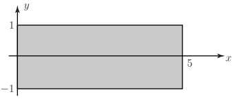
A graph showing a shaded rectangular region bounded by the lines y = 1, y = -1, x = 0, and x = 5.

Long description

Here, the inner integral is

g x = ∫ − 1 1 2 x + y d y

and the outer integral is

I = ∫ x = 0 5 g x d x

Looking in more detail at the inner integral

g x = ∫ − 1 1 2 x + y d y

the function 2 x + y can be integrated with respect to y (keeping x constant) to give 2 x y + 1 2 y 2 + C (where C is a constant and can be omitted as the integral is a definite integral) i.e.

g x = 2 x y + 1 2 y 2 − 1 1 = 2 x + 1 2 − − 2 x + 1 2 = 2 x + 1 2 + 2 x − 1 2 = 4 x .

This is a function of x as expected. This inner integral can be placed into the outer integral to get

I = ∫ x = 0 5 4 x d x

which becomes

I = 2 x 2 0 5 = 2 × 5 2 − 2 × 0 2 = 2 × 25 − 0 = 50

Hence the double integral

I = ∫ x = 0 5 ∫ y = − 1 1 2 x + y d y d x = 50

Key Point 2

Double Integral

When evaluating a double integral, evaluate the inner integral first and substitute the result into the outer integral.

Example 1

Evaluate the double integral I = ∫ x = − 1 2 ∫ y = − 2 3 x 2 y d y d x

This integral is evaluated over the area shown below.

Figure 6
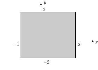
A coordinate plane with a shaded rectangular area defined by the vertices (-2, -1), (2, -1), (2, 3), and (-2, 3).

Long description
Solution

Here, the inner integral is

g x = ∫ y = − 2 3 x 2 y d y = x 2 y 2 2 − 2 3 = 9 2 x 2 − 4 2 x 2 = 5 2 x 2

and hence the outer integral is

I = ∫ x = − 1 2 5 2 x 2 d x = 5 2 1 3 x 3 − 1 2 = 5 6 × 8 − 5 6 − 1 = 15 2

Example 2

Use the above approach to evaluate the double integral

I = ∫ x = 0 5 ∫ y = − 1 1 x 2 cos π y 2 d y d x

Note that the limits are the same as in a previous case but that the function itself has changed.

Solution

The inner integral is

∫ y = − 1 1 x 2 cos π y 2 d y = 2 π x 2 sin π y 2 − 1 1 = 2 π x 2 1 − 2 π x 2 − 1 = 4 π x 2

so the outer integral becomes

I = ∫ x = 0 5 4 π x 2 d x = 4 3 π x 3 0 5 = 4 3 π 125 − 4 3 π 0 = 500 3 π ≈ 53.1

Clearly, variables other than x and y may be used.

Example 3

Evaluate the double integral

I = ∫ s = 1 4 ∫ t = 0 π s sin t d t d s

Solution

This integral becomes (dispensing with the step of formally writing the inner integral),

I = ∫ s = 1 4 − s cos t 0 π d s = ∫ 1 4 − s cos π + s cos 0 d s = ∫ 1 4 − s − 1 + s 1 d s = ∫ 1 4 2 s d s = s 2 1 4 = 16 − 1 = 15

Clearly, evaluating the integrals can involve further tools of integration, e.g. integration by parts or by substitution.

Example 4

Evaluate the double integral

I = ∫ − 1 2 ∫ − 2 3 x y e − x y 2 + 1 d y d x

Here, the limits have not formally been linked with a variable name but the limits on the outer integral apply to x and the limits on the inner integral apply to y . As the integrations are more complicated, the inner integral will be evaluated explicitly.

Solution

Inner integral  = ∫ − 2 3 x y e − x y 2 + 1 d y

which can be evaluated by means of the substitution U = y 2 + 1.

If U = y 2 + 1 then d U = 2 y d y so y d y = 1 2 d U .

Also if y = − 2 then U = 5 and if y = 3 then U = 10.

So the inner integral becomes (remembering that x may be treated as a constant)

∫ 5 10 1 2 x e − x U d U = x e − x 2 ∫ 5 10 d U U = x e − x 2 ln U 5 10 = x e − x 2 ln 10 − ln 5 = x e − x ln 2 2

and so the double integral becomes

I = ∫ − 1 2 x e − x ln 2 2 d x = ln 2 2 ∫ − 1 2 x e − x d x

which can be evaluated by integration by parts.

I = ln 2 2 − x e − x − 1 2 − ∫ − 1 2 1 × − e − x d x = ln 2 2 − 2 e − 2 + − 1 e 1 + ∫ − 1 2 e − x d x = ln 2 2 − 2 e − 2 − e 1 + − e − x − 1 2 = ln 2 2 − 2 e − 2 − e − 1 − e − 2 + e 1 = ln 2 2 − 3 e − 2 ≈ − 0.14
Task!

Evaluate the following double integral.

I = ∫ − 1 1 ∫ 0 2 x 2 y + 3 y 2 d y d x

The inner integral    = ∫ 0 2 x 2 y + 3 y 2 d y = 1 2 x 2 y 2 + y 3 0 2 = 1 2 × 4 x 2 + 8 − ( 0 + 0 ) = 2 x 2 + 8


This can be put in the outer integral to give

I = ∫ − 1 1 2 x 2 + 8 d x = 2 3 x 3 + 8 x − 1 1 = 2 3 + 8 − ( − 2 3 − 8 ) = 4 3 + 16 = 52 3

Exercises

Evaluate the following double integrals over rectangular areas.

  1. I = ∫ x = 0 1 ∫ y = 0 2 x y d y d x
  2. I = ∫ − 2 3 ∫ 0 4 x 2 + y 2 d x d y
  3. I = ∫ 0 π ∫ − 1 1 y sin 2 x d y d x
  4. I = ∫ 0 2 ∫ − 1 3 s t 3 d s d t
  5. I = ∫ 0 3 ∫ 0 1 5 z 2 w w 2 − 1 4 d w d z   (Requires integration by substitution.)
  6. I = ∫ 0 2 π ∫ 0 1 t y sin t d y d t   (Requires integration by parts.)
  1. 1,
  2. 460/3,
  3. 0,
  4. 16,
  5. 9/2,
  6. − π