6 Applications of the normal distribution

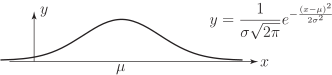
We have, in the previous subsection, noted that the probability density function of a normal distribution $X$ is

$y=\frac{1}{\sigma \sqrt{2\pi }}{e}^{\frac{-{\left(x-\mu \right)}^2}{2{\sigma }^2}}$

This curve is always ‘bell-shaped’ with the centre of the bell located at the value of $\mu$ . The height of the bell is controlled by the value of $\sigma$ . See Figure 10.

Figure 10

We now show, by example, how probabilities relating to a general normal distribution $X$ are determined. We will see that being able to calculate the probabilities of a standard normal distribution $Z$ is crucial in this respect.

Example 11

Given that the variate $X$ follows the normal distribution $X\sim N\left(151,15^2\right)$ , calculate:

1. $\text{P}\left(120\le X\le 155\right)$ ;
2. $\text{P}\left(X\ge 185\right)$

Solution

The transformation used in this problem is $Z=\frac{X-\mu }{\sigma }=\frac{X-151}{15}$

1. $$\begin{array}{rcll}\text{P}\left(120\le X\le 155\right)& =& \text{P}\left(\frac{120-151}{15}\le Z\le \frac{155-151}{15}\right)& \\ & =& \text{P}\left(-2.07\le Z\le 0.27\right)& \\ & =& 0.4808+0.1064=0.5872& \end{array}$$
2. $$\begin{array}{rcll}\text{P}\left(X\ge 185\right)& =& \text{P}\left(Z\ge \frac{185-151}{15}\right)& \\ & =& \text{P}\left(Z\ge 2.27\right)& \\ & =& 0.5-0.4884=0.0116& \end{array}$$

We note that, as for any continuous random variable, we can only calculate the probability that

• $X$ lies between two given values;
• $X$ is greater than a given value;
• $X$ is less that a given value.

rather than for individual values.

Task!

A worn, poorly set-up machine is observed to produce components whose length $X$ follows a normal distribution with mean 20 cm and variance 2.56 cm Calculate:

1. the probability that a component is at least 24 cm long;
2. the probability that the length of a component lies between 19 and 21 cm.

Answer

Example 12

Piston rings are mass-produced. The target internal diameter is 45 mm but records show that the diameters are normally distributed with mean 45 mm and standard deviation 0.05 mm. An acceptable diameter is one within the range 44.95 mm to 45.05 mm. What proportion of the output is unacceptable?

Solution

There are many words in the statement of the problem; we must read them carefully to extract the necessary information. If $X$ is the diameter of a piston ring then $X\sim N\left(45,{\left(0.05\right)}^2\right)$ .

The transformation is $Z=\frac{X-\mu }{\sigma }=\frac{X-45}{0.05}.$

The upper limit of acceptability is $x_2=45.05$ so that $z_2=\left(45.05-45\right)∕0.05=1.$

The lower limit of acceptability is $x_1=44.95$ so that $z_1=\left(44.95-45\right)∕0.05=-1$ .

The range of ‘acceptable’ $Z$ values is therefore $-1$ to 1. Figure 11 below.

Figure 11

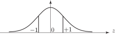
Using the symmetry of the curves $\text{P}\left(-1<Z<1\right)=2\times \text{P}\left(0<Z<1\right)=2\times 0.3413=0.6826.$

Thus the proportion of unacceptable items is $1-0.6826=0.3174,$ or $31.74\%$ .

Example 13

If the standard deviation is halved by improved production practices what is now the proportion of unacceptable items?

Solution

Now $\sigma =0.025$ so that:

$z_2=\frac{45.05-45}{0.025}=2\text{and}{z}_1=-2$

Then $\text{P}\left(-2<Z<2\right)=2\times \text{P}\left(0<Z<2\right)=2\times 0.4772=0.9544$ . Hence the proportion of unacceptable items is reduced to $1-0.9544=0.0456$ or $4.56\%$ .

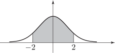
We observe that less of the area under the curve now lies outside the interval $\left(44.95,45.05\right)$ .

Figure 12

Task!

The resistance of a strain gauge is normally distributed with a mean of 100 ohms and a standard deviation of 0.2 ohms. To meet the specification, the resistance must be within the range $100\pm 0.5$ ohms.

1. What percentage of gauges are unacceptable?

   First, state the upper and lower limits of acceptable resistance and find the $Z-$ values which correspond:

   Answer

   $x_1=99.5,x_2=100.5$ $Z=\frac{X-100}{0.2}\left\{{\left(0.2\right)}^2=0.04\right\}$ so that $z_1=-2.5$ and $z_2=2.5$ Now, using a suitable sketch, calculate the probability that $z_1<Z<z_2$ :

   Answer

   

   Long description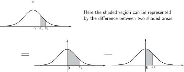

   The shaded area (see diagram) is 0.4938 (from the table of values on page 15). Using symmetry,

   $$\begin{array}{rcll}\text{P}\left(-2.5<Z<2.5\right)& =& 2\times 0.4938& \\ & =& 0.9876.& \end{array}$$

   Hence the proportion of acceptable gauges is $98.76\%$ .

   Therefore the proportion of unacceptable gauges is $1.24\%$ .

2. To what value must the standard deviation be reduced if the proportion of unacceptable gauges is to be no more than 0.2 $\%$ ?

   First sketch the standard normal curve marking on it the lower and upper values $z_1$ and $z_2$ and appropriate areas:

   Answer

   

   Long description

   Now use the Table to find $z_2$ , and hence write down the value of $z_1$ :

   Answer

   $z_2=3.1\text{so that}{z}_1=-3.1$

   Finally, rewrite $Z=\frac{X-\mu }{\sigma }$ to make $\sigma$ the subject. Put in values for $z_2,x_2$ and $\mu$ hence evaluate $\sigma$ :

   Answer

   $\sigma =\frac{X-\mu }{Z}=\frac{100.5-100}{3.1}=0.16\left(2\text{d.p.}\right)$