5 Solving polynomial equations graphically

Polynomial equations, particularly of high degree, are difficult to solve unless they take a particularly simple form. A useful guide to the approximate values of the solutions can be obtained by sketching the polynomial, and discovering where the curve crosses the $x$ -axis. The real roots of the polynomial equation $P\left(x\right)=0$ are given by the values of the intercepts of the function $y=P\left(x\right)$ with the $x$ -axis because on the $x$ -axis $y=P\left(x\right)$ , is zero. Computer software packages and graphics calculators exist which can be used for plotting graphs and hence for solving polynomial equations approximately. Suppose the graph of $y=P\left(x\right)$ is plotted and takes a form similar to that shown in Figure 6.

Figure 6 :

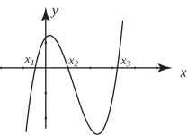
The graph intersects the $x$ axis at $x=x_1$ , $x=x_2$ and $x=x_3$ and so the equation $P\left(x\right)=0$ has three roots $x_1$ , $x_2$ and $x_3$ , because $P\left(x_1\right)=0,P\left(x_2\right)=0$ and $P\left(x_3\right)=0$ .

Example 26

Plot a graph of the function $y=4x^4-15x^2+5x+6$ and hence approximately solve the equation $4x^4-15x^2+5x+6=0$ .

Solution

The graph has been plotted here with the aid of a computer graph plotting package and is shown in Figure 7. By hand, a less accurate result would be produced, of course.

Figure 7 :

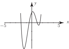
The solutions of the equation are found by looking for where the graph crosses the horizontal axis. Careful examination shows the solutions are at or close to $x=1$ , $x=1.5$ , $x=-0.5$ , $x=-2$ .

An important feature of the graph of a polynomial is that it is continuous . There are never any gaps or jumps in the curve. Polynomial curves never turn back on themselves in the horizontal direction, (unlike a circle). By studying the graph in Figure 6 you will see that if we choose any two values of $x$ , say $a$ and $b$ , such that $y\left(a\right)$ and $y\left(b\right)$ have opposite signs, then at least one root lies between $x=a$ and $x=b$ .

Exercises

1. Factorise $x^3-x^2-65x-63$ given that $\left(x+7\right)$ is a factor.
2. Show that $x=-1$ is a root of $x^3+11x^2+31x+21=0$ and locate the other roots algebraically.
3. Show that $x=2$ is a root of $x^3-3x-2=0$ and locate the other roots.
4. Solve the equation $x^4-2x^2+1=0$ .
5. Factorise $x^4-7x^3+3x^2+31x+20$ given that $\left(x+1\right)$ is a factor.
6. Given that two of the roots of $x^4+3x^3-7x^2-27x-18=0$ have the same modulus but different sign, solve the equation.

   (Hint - let two of the roots be $\alpha$ and $-\alpha$ and use the technique of equating coefficients).

7. Consider the polynomial $P\left(x\right)=5x^3-47x^2+84x$ . By evaluating $P\left(2\right)$ and $P\left(3\right)$ show that at least one root of $P\left(x\right)=0$ lies between $x=2$ and $x=3$ .
8. Without solving the equation or using a graphical calculator, show that $x^4+4x-1=0$ has a root between $x=0$ and $x=1$ .

Answer