4 Further properties of the Fourier transform

We state these properties without proof. As usual F ( ω ) denotes the Fourier transform of f ( t ) .

  1. Time differentiation property:

    F { f ( t ) } = i ω F ( ω )

    (Differentiating a function is said to amplify the higher frequency components because of the additional multiplying factor ω .)

  2. Frequency differentiation property:

    F { t f ( t ) } = i d F d ω or F { ( i t ) f ( t ) } = d F d ω

    Note the symmetry between properties 1. and 2.

  3. Duality property:

    If F { f ( t ) } = F ( ω ) then F { F ( t ) } = 2 π f ( ω ) .

Informally, the duality property states that we can, apart from the 2 π factor, interchange the time and frequency domains provided we put ω rather than ω in the second term, this corresponding to a reflection in the vertical axis. If f ( t ) is even this latter is irrelevant.

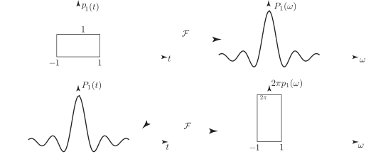
For example, we know that if f ( t ) = p 1 ( t ) = 1 1 < t < 1 0 otherwise , then F ( ω ) = 2 sin ω ω .

Then, by the duality property, since p 1 ( ω ) is even, F { 2 sin t t } = 2 π p 1 ( ω ) = 2 π p 1 ( ω ) .

Graphically:

Figure 6

The image displays two pairs of signals, illustrating the Fourier Transform pair for a rectangular pulse and for a cosine wave.

Long description
Task!

Recalling the Fourier transform pair

  f ( t ) = e 2 t t > 0 e 2 t t < 0 F ( ω ) = 4 4 + ω 2 ,

obtain the Fourier transforms of

  1. g ( t ) = 1 4 + t 2
  2. h ( t ) = 1 4 + t 2 cos 2 t .
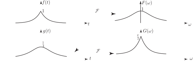
  1. Use the linearity and duality properties:

    We have F { f ( t ) } F { e 2 t } = 4 4 + ω 2 . F { 1 4 e 2 t } = 1 4 + ω 2 (by linearity)

    F { 1 4 + t 2 } = 2 π 1 4 e 2 ω = π 2 e 2 ω = G ( ω ) (by duality).

    The image displays pairs of graphs illustrating the Fourier transform property of time shifting and scaling.

    Long description
  2. Use the modulation property based on the frequency shift property:
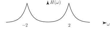
    We have h ( t ) = g ( t ) cos 2 t . F { g ( t ) cos ω 0 t } = 1 2 ( G ( ω ω 0 ) + G ( ω + ω 0 ) ) ,

    so with ω 0 = 2 F { h ( t ) } = π 4 e 2 ω 2 + e 2 ω + 2 = H ( ω )

    A graph showing the real-valued function, denoted as \(H(\omega)\), with two distinct peaks centered symmetrically around the vertical axis.

    Long description
Exercises
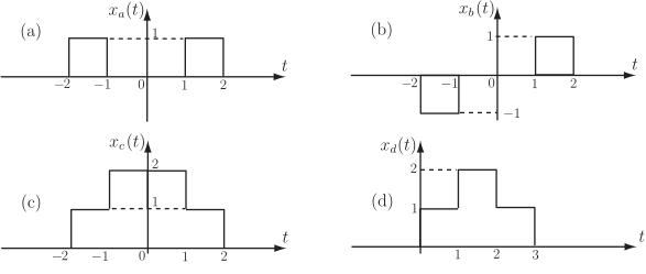
  1. Using the superposition and time delay theorems and the known result for the transform of the rectangular pulse p ( t ) , obtain the Fourier transforms of each of the signals shown.

    The image displays four graphs, labeled (a), (b), (c), and (d), showing time-domain signals \(x_a(t)\), \(x_b(t)\), \(x_c(t)\), and \(x_d(t)\) versus time \(t\).

    Long description
  2. Obtain the Fourier transform of the signal

    f ( t ) = e t u ( t ) + e 2 t u ( t )

    where u ( t ) denotes the unit step function.

  3. Use the time-shift property to obtain the Fourier transform of

    f ( t ) = 1 1 t 3 0 otherwise

    Verify your result using the definition of the Fourier transform.

  4. Find the inverse Fourier transforms of
    1. F ( ω ) = 20 sin ( 5 ω ) 5 ω e 3 i ω
    2. F ( ω ) = 8 ω sin 3 ω e i ω
    3. F ( ω ) = e i ω 1 i ω
  5. If f ( t ) is a signal with transform F ( ω ) obtain the Fourier transform of f ( t ) cos ( ω 0 t ) cos ( ω 0 t ) .
  1. X a ( ω ) = 4 ω sin ( ω 2 ) cos ( 3 ω 2 )

    X b ( ω ) = 4 i ω sin ( ω 2 ) sin ( 3 ω 2 )

    X c ( ω ) = 2 ω [ sin ( 2 ω ) + sin ( ω ) ]

    X d ( ω ) = 2 ω sin ( 3 ω 2 ) + sin ( ω 2 ) e 3 i ω 2

  2. F ( ω ) = 3 + 2 i ω 2 ω 2 + 3 i ω (using the superposition property)
  3. F ( ω ) = 2 sin ω ω e 2 i ω
    1. f ( t ) = 2 2 < t < 8 0 otherwise
    2. f ( t ) = 4 4 < t < 2 0 otherwise
    3. f ( t ) = e t + 1 t < 1 0 otherwise
  4. 1 2 F ( ω ) + 1 4 F ( ω + 2 ω 0 ) + F ( ω 2 ω 0 )