3 Scalar fields

A scalar field is a distribution of scalar values over a region of space (which may be 1D, 2D or 3D) so that a scalar value is associated with each point of space. Examples of scalar fields follow.

1. Figure 2:

   

   Long description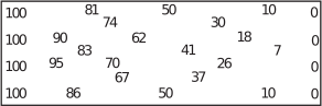

2. Figure 3:

   

   Long description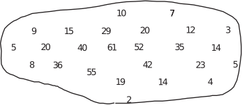
3. The mean annual rainfall at different locations in Britain.
4. The light intensity near a 100 watt light bulb.

To define a scalar field we need to:

• Describe the region of space where it is found (this is the domain )
• Give a rule to show how the value of the scalar is related to every point in the domain.

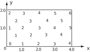
Consider the scalar field defined by $\varphi \left(x,y\right)=x+y$ over the rectangle $0\le x\le 4$ , $0\le y\le 2$ . We can calculate, and plot, values of $\varphi$ at different $\left(x,y\right)$ points. For example $\varphi \left(0,2\right)=0+2=2$ , $\varphi \left(4,1\right)=4+1=5$ and so on.

Figure 4:

Contours

A contour on a map is a curve joining points that are the same height above sea level. These contours give far more information about the shape of the land than selected spot heights.

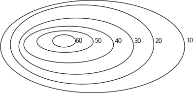
For example, the contours near the top of a hill might look like those shown in Figure 5 where the numbers are the values of the heights above sea level.

In general for a scalar field $\varphi \left(x,y,z\right)$ , contour curves are the family of curves given by $\varphi =c$ , for different values of the constant $c$ .

Figure 5:

Example 6

Describe contour curves for the following scalar fields and sketch typical contours for 1. and 2.

1. $\varphi \left(x,y\right)=x+y$
2. $\varphi \left(x,y\right)=9-x^2-y^2$
3. $\varphi \left(x,y\right)=\frac{1}{x^2+y^2+z^2}$

Solution

1. The contour curves for $\varphi \left(x,y\right)=x+y$ are $x+y=c$ or $y=-x+c$ .
   
   These are straight lines of gradient $-1$ . See Figure 6(a).
2. For $\varphi \left(x,y\right)=9-x^2-y^2$ , the contour curves are $9-x^2-y^2=c$ , or $x^2+y^2=9-c$ . See Figure 6(b). These are circles, centered at the origin, radius $\sqrt{9-c}$ .

   Figure 6:

   

   Long description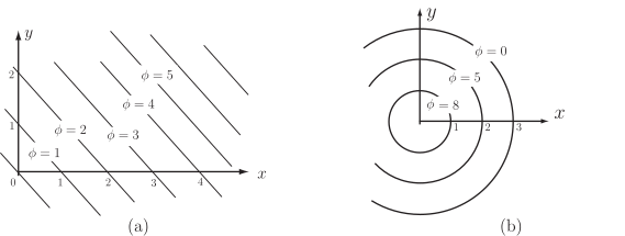
3. For the three-dimensional scalar field $\varphi \left(x,y,z\right)=\frac{1}{x^2+y^2+z^2}$ the contour surfaces are $\frac{1}{x^2+y^2+z^2}=c$ or $x^2+y^2+z^2=\frac{1}{c}$ . These are spheres, centered at the origin and of radius $\frac{1}{\sqrt{c}}$ .

Task!

Describe the contours for the following scalar fields

1. $\varphi =y-x$
2. $\varphi =x^2+y^2$
3. $\varphi =y-x^2$

Answer