1 The gradient of a scalar field

Consider the height $\varphi$ above sea level at various points on a hill. Some contours for such a hill are shown in Figure 14.

Figure 14:

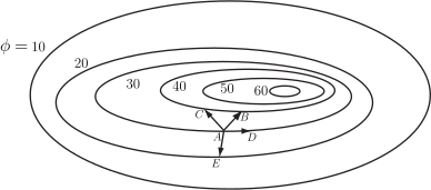
We are interested in how $\varphi$ changes from one point to another. Starting from $A$ and making a displacement $\underset{̲}{d}$ the change in height ( $\varphi$ ) depends on the direction of the displacement. The magnitude of each $\underset{̲}{d}$ is the same.

The change in $\varphi$ clearly depends on the direction of the displacement. For the paths shown $\varphi$ increases most rapidly along $AB$ , does not increase at all along $AD$ (as $A$ and $D$ are both on the same contour and so are both at the same height) and decreases along $AE$ .

The direction in which $\varphi$ changes fastest is along the line of greatest slope which is orthogonal (i.e. perpendicular) to the contours. Hence, at each point of a scalar field we can define a vector field giving the magnitude and direction of the greatest rate of change of $\varphi$ locally.

A vector field, called the gradient, written grad $\varphi$ , can be associated with a scalar field $\varphi$ so that at every point the direction of the vector field is orthogonal to the scalar field contour which is the direction of the maximum rate of change of $\varphi$ .

For a second example consider a metal plate heated at one corner and cooled by an ice bag at the opposite corner. All edges and surfaces are insulated. After a while a steady state situation exists in which the temperature $\varphi$ at any point remains the same. Some temperature contours are shown in Figure 15.

Figure 15:

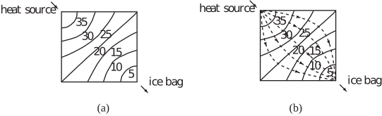
The direction of the heat flow is along the flow lines which are orthogonal to the contours (see the dashed lines in Figure 15(b)); this heat flow is proportional to $\underset{̲}{F}$ = grad $\varphi$ .

Definition
The gradient of the scalar field $\varphi =f\left(x,y,z\right)$ is $\text{grad}\varphi =\underset{̲}{\nabla }\varphi =\frac{\partial \varphi }{\partial x}\underset{̲}{i}+\frac{\partial \varphi }{\partial y}\underset{̲}{j}+\frac{\partial \varphi }{\partial z}\underset{̲}{k}$

Often, instead of grad $\varphi$ , the notation $\underset{̲}{\nabla }\varphi$ is used. ( $\underset{̲}{\nabla }$ is a vector differential operator called ‘del’ or ‘nabla’ defined by $\frac{\partial }{\partial x}\underset{̲}{i}+\frac{\partial }{\partial y}\underset{̲}{j}+\frac{\partial }{\partial z}\underset{̲}{k}$ . As a vector differential operator, it retains the characteristics of a vector while also carrying out differentiation.)

The vector grad $\varphi$ gives the magnitude and direction of the greatest rate of change of $\varphi$ at any point, and is always orthogonal to the contours of $\varphi$ . For example, in Figure 14, grad $\varphi$ points in the direction of $AB$ while the contour line is parallel to $AD$ i.e. perpendicular to $AB$ . Similarly, in Figure 15(b), the various intersections of the contours with the lines representing grad $\varphi$ occur at right-angles.

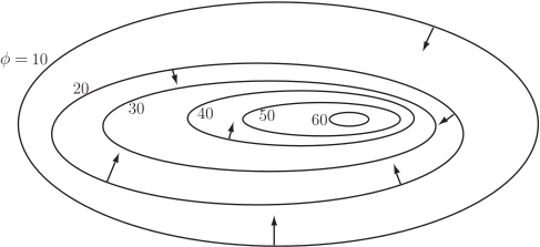
For the hill considered earlier the direction and magnitude of grad $\varphi$ are shown at various points in Figure 16. Note that the magnitude of grad $\varphi$ is greatest (as indicated by the length of the arrow) when the hill is at its steepest (as indicated by the closeness of the contours).

Figure 16:

Example 9

Find grad $\varphi$ for

1. $\varphi =x^2-3y$
2. $\varphi =x{y}^2{z}^3$

Solution

1. grad $\varphi =\frac{\partial }{\partial x}\left(x^2-3y\right)\underset{̲}{i}+\frac{\partial }{\partial y}\left(x^2-3y\right)\underset{̲}{j}+\frac{\partial }{\partial z}\left(x^2-3y\right)\underset{̲}{k}=2x\underset{̲}{i}+\left(-3\right)\underset{̲}{j}+0\underset{̲}{k}=2x\underset{̲}{i}-3\underset{̲}{j}$
2. grad $\varphi =\frac{\partial }{\partial x}\left(x{y}^2{z}^3\right)\underset{̲}{i}+\frac{\partial }{\partial y}\left(x{y}^2{z}^3\right)\underset{̲}{j}+\frac{\partial }{\partial z}\left(x{y}^2{z}^3\right)\underset{̲}{k}=y^2{z}^3\underset{̲}{i}+2xy{z}^3\underset{̲}{j}+3x{y}^2{z}^2\underset{̲}{k}$

Example 10

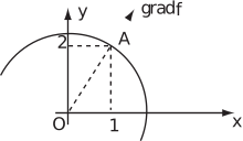
For $f=x^2+y^2$ find grad $f$ at the point $A\left(1,2\right)$ . Show that the direction of grad  $f$ is orthogonal to the contour at this point.

Solution

$\text{grad }f=\frac{\partial f}{\partial x}\underset{̲}{i}+\frac{\partial f}{\partial y}\underset{̲}{j}+\frac{\partial f}{\partial z}\underset{̲}{k}=2x\underset{̲}{i}+2y\underset{̲}{j}+0\underset{̲}{k}=2x\underset{̲}{i}+2y\underset{̲}{j}$

and at $A\left(1,2\right)$ this equals $2\times 1\underset{̲}{i}+2\times 2\underset{̲}{j}=2\underset{̲}{i}+4\underset{̲}{j}$ .

Since $f=x^2+y^2$ then the contours are defined by $x^2+y^2=$ constant, so the contours are circles centred at the origin. The vector grad $f$ at $A\left(1,2\right)$ points directly away from the origin and hence grad $f$ and the contour are orthogonal; see Figure 17. Note that $\underset{̲}{r}\left(A\right)=\underset{̲}{i}+2\underset{̲}{j}=\frac{1}{2}\mathrm{\text{grad}}f$ .

Figure 17:

The change in a function $\varphi$ in a given direction (specified as a unit vector $\underset{̲}{a}$ ) is determined from the scalar product $\left(\text{grad}\varphi \right)\cdot \underset{̲}{a}$ . This scalar quantity is called the directional derivative.

Note:

• $\underset{̲}{a}$ along a contour implies $\underset{̲}{a}$ is perpendicular to $\text{grad}\varphi$ which implies $\underset{̲}{a}\cdot \text{grad}\varphi =0$ .
• $\underset{̲}{a}$ perpendicular to a contour implies $\underset{̲}{a}\cdot \text{grad}\varphi$ is a maximum.

Task!

Given $\varphi =x^2{y}^2{z}^2$ , find

1. grad $\varphi$
2. grad $\varphi$ at $\left(-1,1,1\right)$ and a unit vector in this direction.
3. the derivative of $\varphi$ at $\left(2,1,-1\right)$ in the direction of
   1. $\underset{̲}{i}$
   2. $\underset{̲}{d}=\frac{3}{5}\underset{̲}{i}+\frac{4}{5}\underset{̲}{k}.$

Answer

Exercises

1. Find grad $\varphi$ for the following scalar fields
   1. $\varphi =y-x$ .
   2. $\varphi =y-x^2$ ,
   3. $\varphi =x^2+y^2+z^2$ .
2. Find grad $\varphi$ for each of the following two-dimensional scalar fields given that $\underset{̲}{r}=x\underset{̲}{i}+y\underset{̲}{j}$ and $r=\sqrt{x^2+y^2}$ (you should express your answer in terms of $\underset{̲}{r}$ ).
   1. $\varphi =r$ ,
   2. $\varphi =lnr$ ,
   3. $\varphi =\frac{1}{r}$ ,
   4. $\varphi =r^n$ .
3. If $\varphi =x^3{y}^{2}z$ , find,
   1. $\underset{̲}{\nabla }\varphi$
   2. a unit vector normal to the contour at the point $\left(1,1,1\right)$ .
   3. the rate of change of $\varphi$ at $\left(1,1,1\right)$ in the direction of $\underset{̲}{i}$ .
   4. the rate of change of $\varphi$ at $\left(1,1,1\right)$ in the direction of the unit vector $\underset{̲}{n}=\frac{1}{\sqrt{3}}\left(\underset{̲}{i}+\underset{̲}{j}+\underset{̲}{k}\right)$ .
4. Find a unit vector which is normal to the sphere $x^2+{\left(y-1\right)}^2+{\left(z+1\right)}^2=2$ at the point $\left(0,0,0\right)$ .
5. Find unit vectors normal to ${\varphi }_1=y-x^2$ and ${\varphi }_2=x+y-2$ . Hence find the angle between the curves $y=x^2$ and $y=2-x$ at their point of intersection in the first quadrant.

Answer