7 Straight line graphs
It is often useful to plot graphs of functions to gain an understanding of what they mean. Straight line graphs are produced by linear equations. Linear equations like \(y=2x+4\) only have \(x\) to the power of one only. Note: this doesn’t just apply to \(x\), it could be whatever variable you are using.
7.1 Coordinates
To build a picture of a function we work out pairs of values that satisfy the function. Take for example \(y=\frac{1}{2}x+1\). If we choose values of \(x\) we can work out the corresponding \(y\) values.
| \(x\) | \(y\) |
|---|---|
| \(0\) | \(\frac{1}{2}(0)+1=1\) |
| \(1\) | \(\frac{1}{2}(1)+1=1.5\) |
| \(2\) | \(\frac{1}{2}(2)+1=2\) |
Once we have these values they can be plotted on graph.
The red dots show the points and the blue line shows the equation.
By working out some co-ordinates in the following question try to generate the correct line.
In mathematics, a straight line is technically a special type of curve, just one with no curvature at all. You will often hear mathematicians refer to any line, straight or otherwise, as a “curve”, particularly when its exact shape has not yet been determined.
7.2 The formula for a straight line graph: \(y=mx+c\)
Straight line graphs can be defined by two quantities. The gradient, \(m\), a measure of how steep the line is, and the \(y\) intercept, \(c\), where the line crosses the \(y\) axis.
7.2.1 The y intercept: \(c\)
The \(y\) intercept is where line crosses the \(y\) axis. We can quickly work out the co-ordinate by substituting \(x=0\) into the equation of a line, or, by noticing the constant term in equation where \(y=mx+c\). Here are two examples:
For the line \(y = 3x +4\), the \(y\) intercept is at \((0,4)\) i.e. it crosses the \(y\) axis at \(4\). We can check this by substituting \(x=0\) into the equation.
\[ \begin{aligned} y &= 3x +4 \\ &= 3(0) +4 \\ &= 3\times0 +4 \\ y &= 4 \end{aligned} \]
We need to be careful with the next example: \(y + 2 = 5x\). It’s tempting to say that the \(y\) intercept is \(2\) but it’s not. First we must re-arrange the equation into the form of \(y=mx+c\). We’ll use the idea of doing the same thing to both sides again.
\[ \begin{aligned} y +2 &= 5x \\ y+2-2 &= 5x-2 \\ y &= 5x-2 \end{aligned} \]
Once we’ve done this we can see that the intercept is when \(y=-2\). Notice if we substituted \(x=0\) in the original equaiton we would get this answer too.
\[ \begin{aligned} y +2 &= 5x \\ y+2 &= 5(0) \\ y +2 &= 0 \\ y &= -2 \end{aligned} \]
Click on the graph below and play with the slider for \(c\). Notice how the graph moves up and down.
The graphs and diagrams created in desmos are interactive just click on the edit in desmos button to open the desmos graph in a new tab.
7.2.2 The gradient: \(m\)
The gradient of a graph is a measure of how much steep the line is. The value of \(m\) is the change in the \(y\) axis for each increase of \(1\) in the \(x\) axis. So a gradient of \(m=2\) would mean the \(y\) values increase by \(2\) for each increase of \(1\) in the \(x\) direction. This is a positive gradient. Contrast this to a value of \(m\) such as \(-0.5\). This means for each increase of \(1\) in the \(x\) direction, the corresponding \(y\) value decreases by \(0.5\) or a half. This is a negative gradient.
The gradient can also be found by calculating the change in the \(y\) direction divided by the change in the \(x\) direction. The graph below shows how you could calculate the gradient of the line. The line shown has a gradient of \(\frac{2}{3}\).
A change in a quantity is often represented by the Greek letter delta, \(\Delta\), so we can rewrite \(m\) as: \(m = \frac{\Delta y}{\Delta x}\)
Click on the graph below and then change the value of \(m\) with the slider. Notice how the gradient changes but the \(y\) intercept stays the same.
The graphs and diagrams created in desmos are interactive just click on the edit in desmos button to open the desmos graph in a new tab.
- \(m\) is the gradient - the amount \(y\) changes for an incease in \(1\) in the \(x\) direction
- \(c\) where the line crosses the \(y\) axis
- \(m\) and \(c\) only make sense when the line is in the form \(y=mx+c\)
The equation of a straight line can be written using different letters. They all mean the same thing. You may see:
- \(y = mx + b\)
- \(y = mx + y_0\)
- \(y = ax + b\)
A linear demand curve can be written:
\[ P = 20 - 2Q \] where \(P\) is the price and \(Q\) the quantity.
The intercept \(20\) is the maximum price anyone would pay (when \(Q=0\)). The gradient \(-2\) means that price must fall by \(2\) for each additional unit demanded.
This responsiveness is an example of what economists call elasticity. Here, because we are looking at how quantity demanded responds to a change in price, the specific name is price elasticity of demand. The gradient of the demand curve gives a rough guide: a steep curve means buyers are not very responsive, so demand is inelastic; a flatter curve means buyers are very responsive, so demand is elastic.
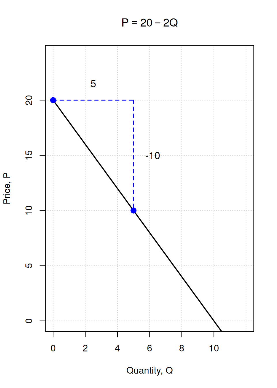
To calculate the gradient we divide the change in the \(y\) direction by the change in the \(x\) direction. Here this is \(\frac{-10}{5} = -2\).
Because the curve slopes downward the gradient is negative, and economists write \(\varepsilon = -2\). Much to the annoyance of mathematicians, they will often drop the minus sign and simply give the positive value, particularly when it is obvious that the gradient is negative.
Using your knowledge of \(y=mx+c\) try the following questions. Don’t be afraid to look at the answers and then try a fresh set of questions if it seems tricky at first.