10 Differentiation
We often want to be able to find the gradient of a curved line. For that we need a new technique, called differentiation, that will give us a rule (a new function) to work out the gradient at any point on the curve.
10.1 The tangent to a curve
The gradient at a point on a curve is the same as the gradient of the tangent at that point. A tangent to a curve is a straight line that just touches curve at that point. Below is a picture of the tangent to the curve when \(x=5\). You can open up the graph and move the point around with the slider.
Notice that the gradient will change depending on which value of \(x\) you use.
10.2 The rules of differentiation
Luckily finding the rule to get the gradient of a curve is straight forward. The language we use for this process is like this. When function is differentiated a new function, the derivative, is found. The derivative enables you to find the gradient. There are lots of ways write this in mathematical notation. Here are the most common.
| original function | derivative |
|---|---|
| \(y\) | \(\frac{dy}{dx}\) |
| \(f(x)\) | \(f'(x)\) |
\(\frac{dy}{dx}\) is pronounced ‘dee \(y\) by dee \(x\)’, and \(f'(x)\) is read as ‘f dash of \(x\)’.
The rule for differentiating polynomials (functions made up of adding different powers of \(x\))is:
- if \(y=ax^n\) then \(\frac{dy}{dx} = anx^{n-1}\), or,
- if \(f(x)=ax^n\) then \(f'(x) = anx^{n-1}\) Times by the power, then take one off the power
Here are some examples:
If \(y = 3x^4\) then \(\frac{dy}{dx} = 3 \times 4 \times x^{4-1} = 12x^3\)
Multiple terms added together are differentiated one by one then added together:
\[ \begin{aligned} y &= 6x^3 + 2x^2 + 4x + 5 \\ &= 6x^3 + 2x^2 + 4x^1 + 5x^0 \\ \frac{dy}{dx} &= 3\times6x^{3-1} + 2\times 2x^{2-1} + 1\times 4x^{1-1} + 0\times5x^{0-1} \\ &= 18x^2 + 4x^1 + 4x^{0} + 0 \\ &= 18x^2 + 4x + 4 \end{aligned} \]
In the above example we’ve used the following mathematical facts:
- \(x=x^1\), \(x\) on it’s own is \(x^1\)
- \(x^0=1\), you can always multiply by \(x^0\) since it’s \(1\)
- \(0 \times a = 0\) anything times zero is zero
The take away from this is that constant terms, terms without \(x\) in, disappear, and terms with just \(x\) in loose the \(x\).
Try these questions to get to grips with the rules of differentiation.
10.3 Finding gradient at a point
To find the gradient at a point. Differentiate the original function and then substitute the \(x\) value of the point into the derivative.
For example to find the gradient when \(x=3\) for the function \(y=x^2\). We would differentiate and then substitute in \(x=3\).
\[ \begin{aligned} y &= x^2 \\ \frac{dy}{dx} &= 2x \\ &= 2(3) \\ &= 2 \times 3 \\ &= 6 \end{aligned} \] So the gradient at \(x=3\) on the curve \(y=x^2\) is \(6\).
If a firm’s total cost of producing \(Q\) units is:
\[ TC = 3Q^2 + 10Q + 50 \]
economists often want to know how much it costs to increase output by one unit when production is already at some specific level. This extra cost is called the marginal cost at that level. It is found by differentiating total cost with respect to quantity and evaluating at the output level in question:
\[ MC = \frac{dTC}{dQ} = 6Q + 10 \]
For example, if the firm is currently producing \(Q = 5\) units, the marginal cost is:
\[ MC = 6(5) + 10 = 40 \]
This means that when output is 5 units, the next unit adds approximately £40 to total cost. The derivative gives the rate of change at a particular point; economists call that rate the marginal cost when it measures the cost of one more unit at the current output level.
Cost functions in economics often involve fractional powers. Suppose a firm’s total cost is:
\[ TC = 5Q^{1.5} + 100 \]
Using the power rule, the marginal cost is:
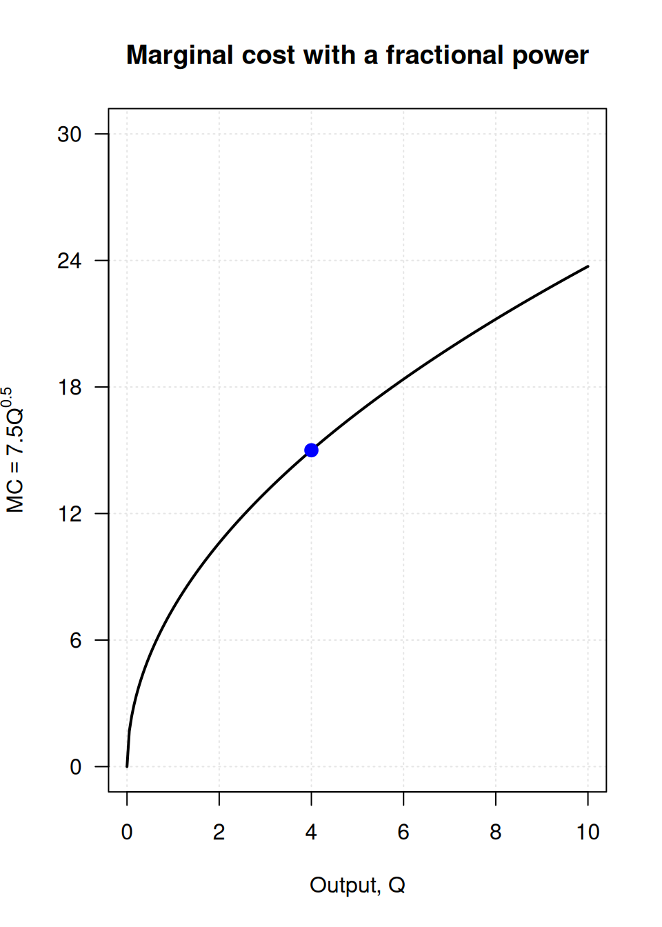
\[ MC = \frac{dTC}{dQ} = 1.5 \times 5 \times Q^{0.5} = 7.5Q^{0.5} \]
Notice that the exponent \(1.5\) becomes \(0.5\). Because the cost function contains a fractional power, the gradient is different at every value of \(Q\). This means marginal cost is not a single number; it depends on where you are on the curve. You must always specify the output level when you quote a marginal cost.
When \(Q = 4\):
\[ MC = 7.5 \times 4^{0.5} = 7.5 \times 2 = 15 \]
So at an output of 4 units, the 5th unit adds approximately £15 to total cost.